What you will make
Read this tutorial on the documentation website or explore the demo gallery for examples, standalone HTML downloads, and complete R scripts.
This tutorial creates a map showing GDP variation, a Florence marriage network, and an FDI map that changes over time. You can customize the controls and legend from R, export independent HTML files, and make an editable static figure.
For a live example of what the package can do, visit FDI Atlas, Keith A. Preble’s interactive website for exploring bilateral foreign direct investment in- and outflows using FDI data provided by UNCTAD. That earlier project helped shape offlineatlas. This tutorial builds standalone examples of related mapping and network workflows.
Publishing an offlineatlas map can be as simple as uploading the
generated .html file to your website and linking to it.
Visitors can explore the map in their browsers without a running R
session or a Shiny server, and they can also download that same file and
open it offline, as well.
FDI Atlas uses a more elaborate hosting arrangement, including a dataset stored in a private folder to prevent data sharing. The offlineatlas examples here embed their mapped data in the HTML itself, so those data are included whenever you share the file (so be mindful of what you share)!
Visiting the hosted FDI Atlas requires an internet connection, but the examples here do not require an internet connection to function (although you will need an internet connection to download and access them).
R prepares the data and writes the necessary files to build the web site. The exported viewers contain all the data, geometry, JavaScript and CSS needed to render the map. Users do not need R, Shiny, a server, an API key or an internet connection. The viewer never retrieves new data, and updates to data sets require rebuilding sites in R when you want to update the underlying observations.
The package API is experimental and a work in progress. This tutorial uses bundled snapshots and does not download data. sf handles geographic inputs, ggplot2 creates static figures, igraph supplies layouts and measures, and ggrepel places labels. These are required R dependencies and are installed automatically when missing during the standard GitHub installation.
install.packages("remotes")
remotes::install_github("preblek/offlineatlas")
Installing R packages require internet access. Systems that build sf from source may also need system libraries or build tools; see the sf installation guide. These authoring dependencies do not change the offline HTML export.
Choose an output folder
For this tutorial, use a temporary folder so running examples does
not write into your project or the installed package. For files you want
to keep, replace output_dir with a folder you own, such as
"my-atlases".
output_dir <- file.path(tempdir(), "offlineatlas-tutorial")
dir.create(output_dir, recursive = TRUE, showWarnings = FALSE)
The examples use overwrite = TRUE so you can rerun them
in this folder. The default for export_html() is
FALSE, which protects existing files.
1. Map a variable across countries
A choropleth colors geographic areas according to a variable. Here, country colors represent GDP per capita in 2024, in current US dollars. These are nominal values, not purchasing-power-adjusted values.
Read the bundled boundaries and GDP snapshot. Join by a stable
country ID, not by row order or the spelling of a country name.
match() returns NA for an unmatched ID. Keep
those rows so their boundaries remain on the map.
world <- sf::st_read(example_file("world_sf.geojson"), quiet = TRUE)
gdp <- example_data("worldbank_gdp")
stopifnot(!anyDuplicated(gdp$id))

joined <- match(world$id, gdp$id)
world$gdp <- gdp$gdp_per_capita[joined]
world$matched <- !is.na(joined)
matched distinguishes a country without a matching
source record from a matched record whose GDP value is unavailable. Both
appear as missing on the map, but details and data downloads preserve
the distinction. No missing value is replaced with zero.
Start with atlas(), then add the geographic data with
add_areas(). Column names are quoted strings.
values selects the variable to color, and
labels supplies its reader-facing name.
gdp_map <- atlas(
  "GDP per capita in 2024",
  units = "USD",
  entity_name = "country", entity_names = "countries",
  notice = "Current US dollars. Missing observations are not imputed.",
  sources = c(
    "World Bank WDI, 2024 snapshot, CC BY 4.0.",
    "Natural Earth boundaries, public domain."
  )
) |>
  add_areas(
    world, id = "id", label = "label",
    values = "gdp", labels = "GDP per capita (USD)",
    matched = "matched",
    breaks = list(c(1000, 5000, 15000, 40000, 80000))
  )

export_html(gdp_map, file.path(output_dir, "gdp.html"), overwrite = TRUE)
Five breakpoints create six color intervals. A value exactly on a
breakpoint belongs to the higher interval, so 5,000 belongs to the
interval beginning at 5,000. Missing values have their own legend key.
The breaks argument is a list because an area map can
expose more than one variable.
Open the exported file directly in a browser. In an interactive R session, you can also use the following command.
For your own map, use sf::st_read() to read local
boundaries, join your variables by identifiers, and pass the resulting
sf object to add_areas(). Polygon and
multipolygon geometry is also supported. A valid CRS must be present;
projected inputs are transformed during preparation. The HTML display
uses a fixed equirectangular projection with latitude coverage from -60
to 85. Invalid shapes and out-of-range geometry produce errors. Repair
or clip them explicitly before mapping. The package does not guess a CRS
or silently remove features.
Inspect the data before exporting
summary() reports what is actually in the atlas. It
separates matched records with missing values from areas with no
matching record, and keeps zero and negative values distinct. The result
contains ordinary data frames that you can inspect or save.
audit <- summary(gdp_map)
audit$areas
#>   variable                label    type time total observed missing unmatched
#> 1      gdp GDP per capita (USD) numeric <NA>   176      162      14         7
#>   unavailable negative zero positive
#> 1           7        0    0      162
missing includes both unmatched and
unavailable, so do not add those three columns together.
For a timeline, areas contains one row per variable and
period. categories counts every declared category,
including unused ones. relationships reports supplied ties
by period and layer. Numeric sign counts are NA for
categories and unweighted networks. The summary cannot recover source
records that you removed before creating the atlas.
Frame a region automatically
Call set_view() without bounds to fit the supplied
geographic data. This example uses the bundled European boundaries for
Belgium, the Netherlands and Luxembourg. Its values are joined from the
same GDP snapshot.
europe <- sf::st_read(example_file("europe_sf.geojson"), quiet = TRUE)
region <- europe[europe$id %in% c("BEL", "NLD", "LUX"), ]
joined <- match(region$id, gdp$id)
region$gdp <- gdp$gdp_per_capita[joined]
region$matched <- !is.na(joined)
regional_map <- atlas(
  "GDP per capita in the Benelux countries", units = "USD",
  sources = "World Bank WDI, 2024 (CC BY 4.0); Natural Earth (public domain)."
) |>
  add_areas(region, label = "label", values = "gdp", matched = "matched",
            breaks = list(c(40000, 80000))) |>
  set_view(title = "Benelux", padding = 0.05) |>
  set_preset("compact")
export_html(regional_map, file.path(output_dir, "regional-gdp.html"),
            overwrite = TRUE)
Add all geographic layers before fitting. The function includes every supplied feature, even if its value is missing. It preserves islands and outlying territories, so subset the geometry explicitly when you want only a particular region to display. However, please note that it does not change projection. Very small regions have a minimum one-degree span, and dateline-crossing geometry can require a world view. With sf boundaries, the package can automatically fit the map to your region. If you supply SVG shapes instead, specify the viewing area using west, south, east, and north coordinates.
2. Draw the Florence marriage network
Networks use a table of entities and a table of relationships. Node IDs must be unique. Both endpoints of each relationship must match a node ID.
The Florence fixture includes marriage and business relationships. Select only marriage ties for this example. Family positions are a supplied schematic layout, not historical residential locations.
families <- example_data("florence_nodes")
ties <- example_data("florence_edges")
marriages <- ties[ties$layer == "Marriage", ]
# A display category derived from the name, not a historical measurement.
families$family_role <- ifelse(families$label == "Medici", "Medici", "Other families")
stopifnot(nrow(marriages) > 0)
marriage_map <- atlas(
  "Marriage alliances in Florence",
  entity_name = "family", entity_names = "families",
  notice = paste(
    "Teaching subset. Positions show network structure,",
    "not historical residences."
  ),
  sources = c(
    "Padgett / CoMuNe Lab Florentine families data.",
    "Database ODbL 1.0; individual contents DbCL 1.0.",
    "https://github.com/CoMuNeLab/Padgett-Florentine-Families",
    "https://opendatacommons.org/licenses/odbl/1-0/",
    "https://opendatacommons.org/licenses/dbcl/1-0/",
    "Expanded family names and rescaled supplied schematic coordinates."
  )
) |>
  add_nodes(
    families, id = "id", label = "label",
    layout_x = "x", layout_y = "y", coordinates = "schematic",
    attributes = "family_role"
  ) |>
  add_edges(
    marriages, from = "from", to = "to", layer = "layer",
    directed = FALSE, coverage = "edge_list"
  )

export_html(marriage_map, file.path(output_dir, "florence.html"),
            overwrite = TRUE)
Read the full source and license notice with
readLines(example_file("FLORENCE-NOTICE.txt")). Keep those
notices when redistributing the data. This example is a teaching subset,
not the complete network from the original study.
To compare marriage and business layers, supply ties
instead of marriages in a new atlas
construction. Nodes, relationships and areas can each be added once.
Supply schematic coordinates, or omit them and call
layout_network() after adding edges. For geographic
networks, add_nodes() accepts longitude and latitude
columns or sf POINT geometry.
For weighted flows, use weight with
coverage = "observed_rows", or a complete directed panel
with coverage = "complete_panel" and a time column. An
omitted observed row is not assumed to be zero. Negative weights require
signed = TRUE.
The add_edges() help page explains how to specify whether your data lists connections, contains only observed records, or includes every expected combination, and how missing records are handled.
3. Add an FDI timeline
A numeric area timeline has one row per country and period. Every
period must have the same IDs, labels and geometry. Values, matching
status and notes can change. Include explicit NA
observations for missing values.
Use the bundled national inward FDI snapshot for 1990-2025. Units are millions of current US dollars. Negative flows, reported zeroes and unavailable values remain distinct. The separate bilateral FDI fixture is not used here, and its sample flows must not be treated as national totals.
These UNCTAD Data Hub data use CC BY 3.0 IGO. Read
readLines(example_file("FDI-NOTICE.txt")) for the source
and adaptations, and retain attribution and the license link in shared
outputs. The Data
Hub reuse terms apply to these data separately from the package’s
MIT software license.
# Start with a fresh boundary table, without the GDP attributes.
boundaries <- sf::st_read(example_file("world_sf.geojson"), quiet = TRUE)
fdi <- example_data("fdi_national")
periods <- sort(unique(fdi$year))

frames <- lapply(periods, function(period) {
  records <- fdi[fdi$year == period, ]
  stopifnot(!anyDuplicated(records$id[nzchar(records$id)]))
  joined <- match(boundaries$id, records$id)
  frame <- boundaries
  frame$year <- period
  frame$matched <- !is.na(joined)
  frame$inflow <- records$inflow_usd_millions[joined]

  # Preserve missing-data reasons and source footnotes in each period.
  frame$note <- vapply(joined, function(j) {
    if (is.na(j)) return("No matching source record for this area and year.")
    parts <- c(records$inflow_usd_millions_missing_reason[j],
               records$inflow_usd_millions_footnote[j])
    paste(parts[!is.na(parts) & nzchar(parts)], collapse = ". ")
  }, character(1))
  frame
})
observations <- do.call(rbind, frames)
Creating each frame from the same boundary table preserves the
complete roster and fixed geometry. Countries without records stay in
the panel with NA values. Historical economy identifiers
are not reassigned to successors.
fdi_map <- atlas(
  "FDI inflows over time", units = "USD millions",
  entity_name = "country or area", entity_names = "countries and areas",
  notice = paste(
    "Annual inward flows, current USD millions. Negative values and zeroes",
    "are retained. Present-day boundaries are used in every period;",
    "historical economies are not reassigned. Revision status is not supplied."
  ),
  sources = c(
    "UNCTAD Data Hub, FDI flows and stock. CC BY 3.0 IGO.",
    "https://creativecommons.org/licenses/by/3.0/igo/",
    "National inward flows, 1990-2025; regional aggregates excluded.",
    "Natural Earth boundaries, public domain. No UN endorsement is implied."
  )
) |>
  add_areas(
    observations, id = "id", label = "label",
    values = "inflow", labels = "FDI inflows (USD millions)",
    time = "year", matched = "matched", notes = "note",
    breaks = list(c(-10000, 0, 1000, 10000, 100000)),
    colors = list(c("#a9602d", "#e4b87e", "#edf4db",
                    "#8fc1a0", "#247577", "#164c60"))
  ) |>
  set_controls(initial_time = "2025")

export_html(fdi_map, file.path(output_dir, "fdi-timeline.html"),
            overwrite = TRUE)
Open the file, choose a year, or use Previous, Play and Next. Color intervals stay fixed across years. Playback advances between supplied observations at equal intervals, without interpolation. Select exactly one country to reveal its numeric history chart and table. Missing values break the line; zero and negative observations remain visible. The history scale stays fixed for the selected country across playback, but can differ between countries.
The same panel structure supports categorical timelines such as EU
enlargement. Supply categories = list(levels) and an
explicit color vector through colors, with
time = "year". Categorical colors retain their meaning
throughout the series. Categorical variables do not produce a numeric
history chart. The installed examples/eu.R script contains
the full enlargement example, using present-day boundaries and
documented membership dates.
4. Customize controls, legends and fonts
Start with a reusable preset when you want coordinated defaults.
compact uses smaller legend keys and tighter spacing;
presentation uses larger text and keys. Both use local
sans-serif fonts and preserve data, labels, source notes, initial
filters and control visibility.
compact_map <- set_preset(fdi_map, "compact")
presentation_map <- set_preset(fdi_map, "presentation")
Presets set layout fields, including toolbar position, legend placement and fonts. Use them before your own overrides. Static legends choose a column count based on category count and label length unless you set one explicitly. You still choose figure width and height when saving with ggplot2.
You can make presentation changes in R without editing JavaScript or CSS directly. In this example, keep the initial year explicit, move the toolbar, slow playback, and provide readable labels for the six fixed FDI intervals.
custom_map <- fdi_map |>
  set_controls(
    initial_time = "2025", position = "above_map", playback_interval = 1800,
    visible = c(search = TRUE, downloads = TRUE),
    labels = c(play = "Animate", pause = "Pause", "next" = "Later")
  ) |>
  set_legend(
    title = "Annual inward FDI", position = "below", columns = 2,
    missing_label = "Unavailable or unmatched",
    labels = list(inflow = c(
      "<-10,000", "-10,000 to <0", "0 to <1,000",
      "1,000 to <10,000", "10,000 to <100,000", "\u2265100,000"
    ))
  ) |>
  set_style(font_family = "sans", heading_family = "sans")

export_html(custom_map, file.path(output_dir, "fdi-customized.html"),
            overwrite = TRUE)
Legend aliases change display text only. Original values remain in data exports. Labels are plain text. Fonts come from the viewing computer and are not downloaded, so exact appearance may vary.
Each configuration function replaces its own previous settings with
its arguments and defaults. Keep the desired options together in one
call. For example, when changing playback speed, repeat
initial_time if you want to retain a previously configured
starting period. A control appears only when relevant to the supplied
data, even if requested as visible. Hiding controls does not remove data
from the HTML.
To start on Europe, use
set_view(custom_map, c(-25, 33, 45, 72)). To add one
separate detail panel, use
set_inset(custom_map, c(-15, 34, 35, 62), title = "Europe detail").
Bounds are west, south, east and north. Both functions return an updated
atlas, so assign the result before exporting. Regional framing does not
change the map projection, and dateline-crossing bounds are
unsupported.
5. Make a static figure with ggplot2
An atlas built from sf polygons can also become an
ordinary ggplot object. Choose an original variable column name and, for
a timeline, one period. The static map preserves interval boundaries,
colors, missing values and legend aliases. Add normal ggplot2 themes,
labels or layers afterwards.
p <- as_ggplot(set_preset(custom_map, "compact"),
               variable = "inflow", time = 2025) +
  ggplot2::labs(
    title = "FDI inflows in 2025",
    subtitle = "Millions of current US dollars"
  ) +
  ggplot2::guides(fill = ggplot2::guide_legend(
    title = NULL, ncol = 4, byrow = TRUE
  )) +
  ggplot2::theme(
    legend.position = "bottom",
    legend.text = ggplot2::element_text(size = 8),
    legend.key.size = grid::unit(3, "mm")
  )
# Wrap the retained source caption to fit this figure's width.
p <- p + ggplot2::labs(
  caption = paste(strwrap(p$labels$caption, width = 80), collapse = "\n")
)
p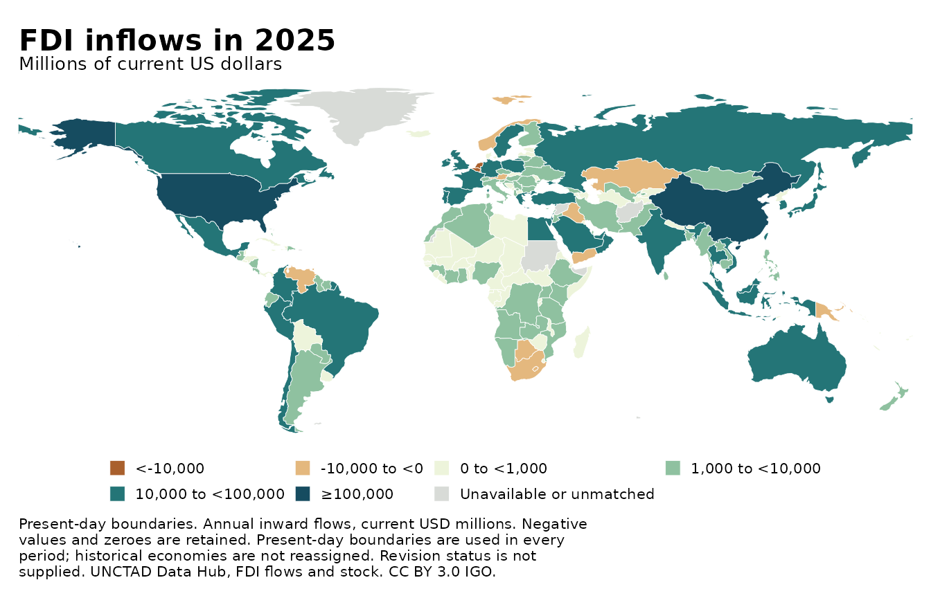
The static legend is adjustable. guide_legend(ncol = 4)
makes two compact rows for these seven keys. legend.text
sets label size and legend.key.size sets swatch size.
guide_legend(title = NULL) removes the redundant legend
title; the subtitle already gives the units. Use
legend.position = "right" to move the legend, or
"none" to hide it. These ggplot2 changes apply to this
static figure without changing the interactive atlas.
An interval labeled 0 to <1,000 includes values from zero up to, but not including, 1,000. A label such as ≥80,000 means 80,000 or more.
Static output also supports schematic and geographic networks. It
does not reproduce browser selection, history charts or the browser’s
current zoom. Visible insets and illustrated SVG backgrounds are omitted
with a warning. Area maps and geographic network boundaries require
sf input, and prepared SVG path tables do not retain the
required geometry.
Make a static network figure
Use the Florence atlas built earlier. Here an automatic layout replaces the supplied schematic positions, symbol size shows distinct marriage partners, and fill distinguishes Medici from the other families. All families, including isolates, are retained. A minimum symbol size keeps zero values visible.
marriage_figure <- as_ggplot(set_preset(marriage_map, "compact"),
                           layers = "Marriage", layout = "fr", seed = 7,
                           node_size_by = "degree", node_fill_by = "family_role") +
  ggplot2::labs(title = "Marriage alliances in Florence") +
  ggplot2::scale_fill_manual(name = "Family",
    values = c("Medici" = "#b46c3b", "Other families" = "#177b7b"))
#> Scale for fill is already present.
#> Adding another scale for fill, which will replace the existing scale.
marriage_figure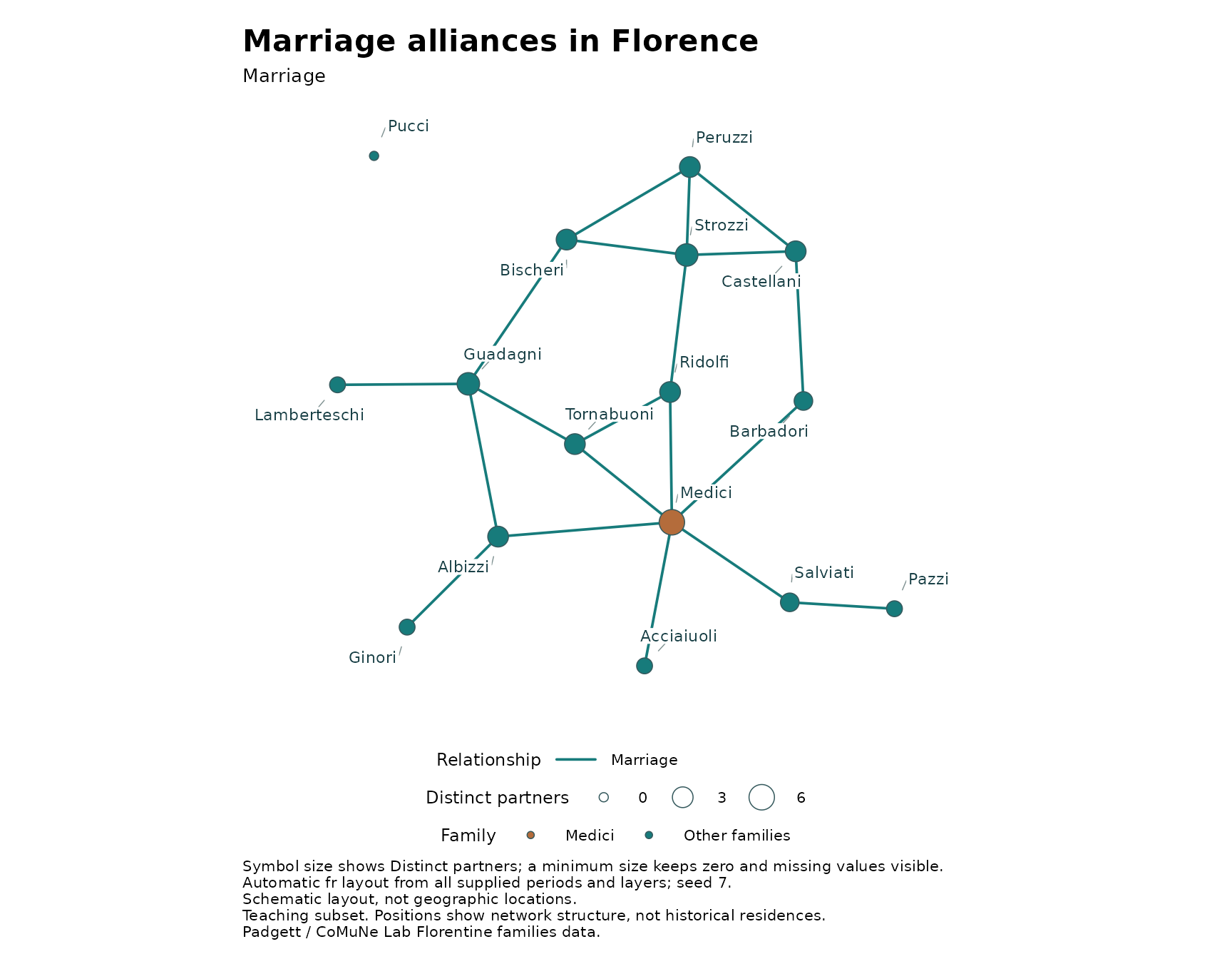
ggplot2::ggsave(file.path(output_dir, "florence-marriages.png"),
               marriage_figure, width = 9, height = 7, dpi = 200)
For a network containing several relationship layers,
layers = "Marriage" shows one layer and
layers = c("Marriage", "Business") shows both. Colors
remain stable as you change the selected layers.
labels = FALSE hides node labels. By default, ggrepel
places labels away from other labels and symbols, with leader lines.
Labels within the map bounds are retained, although very crowded figures
may need more space. Use repel = FALSE for simple offset
labels.
The "fr" layout uses Fruchterman-Reingold. Alternatives
are "kk" (Kamada-Kawai) and "circle";
"existing" keeps supplied positions. Layouts ignore
direction and weight magnitude and use all supplied periods and layers
to keep positions stable across filters. Geographic locations are never
moved by these layout algorithms. Seeds make layouts and labels
reproducible with the same library versions, fonts and figure
dimensions.
For a layout shared by HTML and static figures, calculate it on the atlas:
arranged_marriages <- layout_network(marriage_map, "fr", seed = 7)
export_html(arranged_marriages, file.path(output_dir, "florence-automatic.html"),
            overwrite = TRUE)
You can also omit both schematic coordinate columns in
add_nodes() to start from a circle, then call
layout_network() after adding edges. The coordinates are
calculated in R and saved in the HTML. The exported viewer does not need
igraph or an R session and does not recalculate the layout.
Use attributes in add_nodes() to retain
your own numeric or categorical columns. They remain in R for static
styling and are excluded from the HTML payload.
node_size_by accepts a nonnegative numeric column;
node_fill_by accepts numeric or categorical columns;
node_shape_by accepts up to five categories. The Florence
example retained family_role for this purpose. Missing
fills are gray; missing shape categories use crosses. Missing and zero
size values receive a minimum-size symbol while their original values
stay distinct in the plot data.
Built-in measures are degree, in_degree,
out_degree, strength,
in_strength, out_strength,
betweenness, and component. Degree counts
distinct observed partners. Strength sums known absolute weights; the
strength_partial and corresponding incoming/outgoing flags
identify incomplete totals. All-missing supplied records yield NA.
Betweenness ignores weight magnitudes. Measures use the current year,
layers and source filters. Node scales adapt to each figure, so set
fixed ggplot2 scale limits yourself when comparing periods. You can
adjust titles, legends, palettes, size ranges, shapes and themes with
ordinary ggplot2 functions.
Geographic networks use the same function. Supply any background
boundaries as sf polygons. For a directed network, choose a
year and optionally a source:
source(system.file("examples", "aid.R", package = "offlineatlas"))
aid_figure <- as_ggplot(aid_atlas, time = 2024, source = "CAN")
ggplot2::ggsave("canada-aid-2024.png", aid_figure,
                width = 9, height = 7, dpi = 200)
With source = NULL, every source is included,
independently of the HTML initial-source setting. Directed ties have
arrows along their paths. Line width shows absolute weight on a fixed
scale across all supplied periods and layers; negative values use dashed
lines without reversing their direction. Zero and unavailable rows
produce no lines and remain distinct in
attr(aid_figure, "offlineatlas_edges"). All nodes stay
visible after filters. Geographic lines are schematic connections, with
dateline splitting, not travel routes. The returned plot’s
data contains the node table.
The installed examples/static_networks.R script saves
both schematic and geographic network figures as PNG, PDF and SVG.
Share and inspect the results
The six HTML files can be opened directly and shared independently. The example code below lists them without launching a browser during a build. Temporary files may be removed when your R session ends. Copy the files you want to keep to a permanent folder.
list.files(output_dir, pattern = "[.]html$")
#> [1] "fdi-customized.html"     "fdi-timeline.html"
#> [3] "florence-automatic.html" "florence.html"
#> [5] "gdp.html"                "regional-gdp.html"
The viewer offers several downloads.
- SVG and PNG capture the current map or network, including captions, the legend, and any visible inset or numeric history chart.
- View data CSV follows the current filters and selection.
- History CSV contains every period for the selected country.
- All data JSON includes all embedded periods and mapped data, regardless of which controls are hidden. It also retains the prepared node coordinates.
Static figures can also be saved as PDFs in R. PDF download links are planned for the demo gallery.
figure <- as_ggplot(my_atlas)

ggplot2::ggsave(
  "my-figure.pdf",
  plot = figure,
  width = 9,
  height = 6,
  units = "in"
)
Replace my_atlas with the name of your atlas object.
This saves a 9-by-6-inch PDF in your working directory.
Search narrows the selection list but not the underlying map data. Clear focus restores all entities while retaining filters and zoom. Exporting a current view pauses playback. CSV text that could be interpreted as a spreadsheet formula receives a protective apostrophe; JSON preserves the original text.
For the complete API, use help(package = "offlineatlas")
and the individual function pages, especially ?add_areas,
?add_edges, ?set_controls and
?export_html. The package overview is available with
?offlineatlas.